Introduction to CAPM
- The Capital Asset Pricing Model is a mathematical model used to estimate the expected return of an investment based on its risk level relative to the market.
- Goal is to Check if stock is fairly valued taking into account its risk and time value of money.
- He identified two types of risk
- systematic: Also called market risk. It is influenced by factors such as interest rates, inflation, recessions and geopolitical events like war. all assets are impacted in similar ways.
- unsystematic: these are risks that are unique to each asset.
- The capital asset pricing model concentrates on measuring systemic risk and its impact on the value of an asset.
- CAPM helps factor in systemic risks to estimate the fair value of an asset and understand the relationship between risk and expected returns.
- Shows relationship between systematic risk and expected returns.
- Based on beta, risk free rate, market risk premium.
- Widely used for pricing risky securities because its simple and allows easy comparisons.
- Used in conjuction with MPT to understand portfolio risk and expected returns.
- The CAPM was developed in the early 1960s by Financial Economist William Sharpe who built his work on the ideas put forth by Harry Markowitz.
Basic Theory
- Key Terms for CAPM
- Expected Return: It is a well-grounded estimate of the returns an investor can expect over the life of an investment.
- Risk Free Rate: The rate of return an investor would expect from an asset that bears no risk.
- In india it is taken as the 10 year government bond yield since they are backed by the full faith and credit of the Indian Government.
- As of Dec 23, 2022 it is 7.33%
- Beta: It quantifies the riskiness (volatility) of a stock compared with the market.
- \(=1\)
- \(<1\)
- >1
- Market Risk Premium: Historical returns generated by a comparable market.
- Briefly put, the CAPM model generates the expected returns of assets given the risk of those assets. This is known as risk-adjusted expected return.
- The formula is as follows:
\[ER_i = Rf + \beta \times [ER_m - Rf]\]
where \(ER_i\) = Expected Return of Asset
\(Rf\) = Risk Free rate is the rate of return of an asset with zero risk. In india it is taken as the 10 year government bond yield. 7.33%
\(\beta\) = Beta Value of Stock. It quantifies the riskiness (volatility) of a stock compared with the market.
\(ER_m\) = market premium. Returns generated by market for given tenure.
Usecases
- Importance of beta of companies for investors
- The CAPM plays a key role in financial modeling and asset valuation
- While valuing a stock, an investor uses WACC to find NPV of future cash flows. CAPM is used to calculate cost of equity in calculation of WACC.
- CAPM formula is still widely used because it is simple and allows for easy comparisons of investment alternatives.
- Used as a tool combined with other methods of evaluating securities, it can play an integral role in helping investment professionals make informed investment decisions.
- it is used in conjunction with modern portfolio theory (MPT) to understand portfolio risk and expected returns.
How is CAPM useful for Investors
Shortfalls (limitations)
- Assumes that risk free rate remains constant. Over an analyst’s chosen investment time horizon, the risk-free rate can fluctuate
Practical Example (In Indian Context) with Python Code with code outputs
Getting Data
#importing required libraries
import yfinance as yf

import pandas as pd

import matplotlib.pyplot as plt

import numpy as np

import plotly.express as px

from sklearn.linear_model import LinearRegression

#getting historic stock data from yfinance
stocks_list = ['BHARTIARTL.NS', 'ITC.NS', 'HDFCBANK.NS','^NSEI']

data = yf.download(stocks_list, period='5y')['Adj Close']

data.columns = ['BHARTIARTL','HDFCBANK', 'ITC','NIFTY_50']
EDA of historic Data
Normalize stock prices (so easy to compare)
- Visualise all historic prices (normalized)
#Normalizing Stock Prices

def normalize_prices(df):

    df_ = df.copy()

    for stock in df_.columns:

        df_[stock] = df_[stock]/df_[stock][0]

    return df_

norm_df = normalize_prices(data)

# Plotting the normalized stock prices

fig = px.line(title = "Normalized stock prices")

for stock in norm_df.columns:

    fig.add_scatter(x = norm_df.index.values, y = norm_df[stock], name = stock)

fig.show()
Calculating Daily Returns (%)
# Calculating Daily % change in stock prices

daily_returns = norm_df.pct_change()

daily_returns.iloc[0,:] = 0

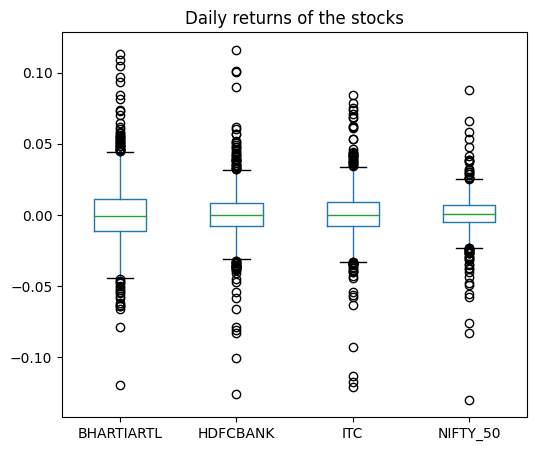
# Boxplot of daily returns (in %)

daily_returns.boxplot(figsize=(6, 5), grid=False)

plt.title("Daily returns of the stocks")
Interpreting the results
CAPM Model
# Initializing empty dictionaries to save results

beta,alpha = dict(), dict()

# Make a nice subplot

fig, axes = plt.subplots(1,3, dpi=150, figsize=(15,8))

axes = axes.flatten()

# Loop on every stock daily return

for idx, stock in enumerate(daily_returns.columns.values[:-1]):

    # scatter plot between stocks and the NSE

    daily_returns.plot(kind = "scatter", x = "NIFTY_50", y = stock, ax=axes[idx])

    # Fit a line (regression using polyfit of degree 1)

    b_, a_ = np.polyfit(daily_returns["NIFTY_50"] ,daily_returns[stock], 1)

    regression_line = b_ * daily_returns["NIFTY_50"] + a_

    axes[idx].plot(daily_returns["NIFTY_50"], regression_line, "-", color = "r")

    # save the regression coeeficient for the current stock

    beta[stock] = b_

    alpha[stock] = a_

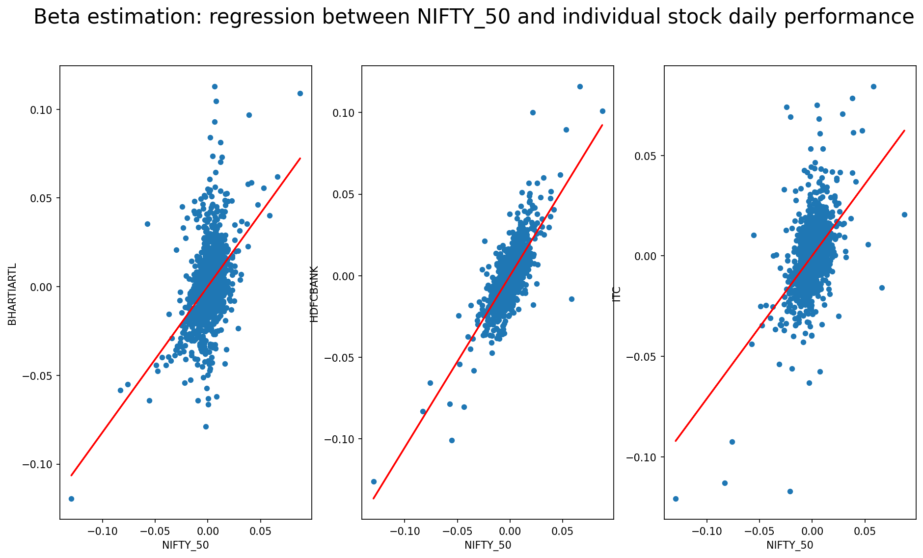
plt.suptitle("Beta estimation: regression between NIFTY_50 and individual stock daily performance", size=20)

plt.show()
The plot generated by the code is a scatterplot with a linear regression line superimposed on top of it. The scatterplot shows the relationship between the daily returns of the NIFTY_50 index and the daily returns of an individual stock. The regression line shows the overall trend in this relationship.
By looking at the slope of the regression line, you can determine the beta of the individual stock. Beta is a measure of a stock’s volatility in relation to the overall market. A beta of 1 means that the stock’s price moves in line with the market, while a beta less than 1 means that it is less volatile than the market, and a beta greater than 1 means that it is more volatile.
You can also determine the alpha of the individual stock from the intercept of the regression line. Alpha is a measure of the stock’s performance relative to the market. A positive alpha indicates that the stock has outperformed the market, while a negative alpha indicates that it has underperformed the market.
You can use the beta and alpha values to compare the relative risk and return of different stocks, and to make informed investment decisions.
Calculating Beta
keys = list(beta.keys())
beta_3 = dict()

for k in keys:

beta_3[k] = [daily_returns[[k,'NIFTY_50']].cov()/daily_returns['NIFTY_50'].var()][0].iloc[0,1]- Explaining beta in terms of Regression between market and stock
- Visualize the regression line #### calculate expected return of stock prices with actual historic returns
# Initialize the expected return dictionary

ER = dict()

rf = 0.0733

trading_days = 250

# Estimate the expected return of the market using the daily returns

rm = daily_returns["NIFTY_50"].mean() * trading_days

for k in keys:

    # Calculate return for every security using CAPM

    ER[k] = rf + beta[k] * (rm-rf)

for k in keys:

    print("Expected return based on CAPM model for {} is {}%".format(k, round(ER[k]*100, 2)))

# Calculating historic returns

for k in keys:

    print('Return based on historical data for {} is {}%'.format(k, round(daily_returns[k].mean() * 100 * trading_days, 2)))

Conslusion
- The CAPM uses the principles of modern portfolio theory to determine if a security is fairly valued.
- It relies on assumptions about investor behaviors, risk and return distributions, and market fundamentals that don’t match reality.
- However, the underlying concepts of CAPM and the associated efficient frontier can help investors understand the relationship between expected risk and reward as they strive to make better decisions about adding securities to a portfolio.